Our Location
No.503 Xingguo Road, Yuhang Economic and
Technological Development Zone, Hangzhou

No.503 Xingguo Road, Yuhang Economic and
Technological Development Zone, Hangzhou

A practical method for calculating energy meter test bench system uncertainty using repeatability, resolution, and reference standard uncertainty with k=2.
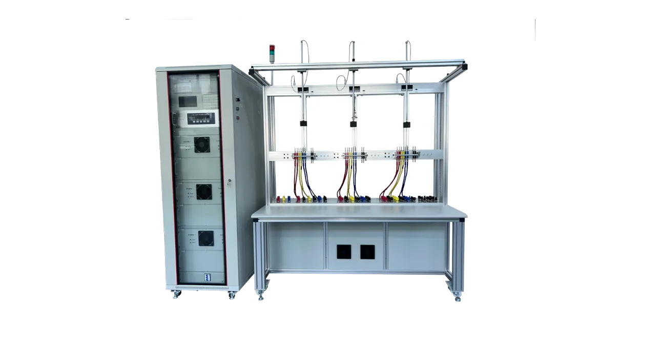
System uncertainty is one of the most important results produced by an energy meter test bench. It describes how reliably the test bench can determine the error of a meter under test and provides the context needed to compare that error with the applicable acceptance limit.
This article presents a practical calculation method based on repeated measurements, display resolution, and the calibration certificate of the reference standard meter. The worked example and 24-point summary are based on an actual test-bench uncertainty calculation workbook for a three-phase energy meter test system.
A test bench may show a meter error of 0.001% or 0.003%, but the meaning of that value depends on the uncertainty of the complete measurement system. A reference standard, source, meter connection, pulse input, display resolution, environmental conditions, and repeatability all contribute to the result.
Without a documented uncertainty budget, a pass/fail decision can be misleading. A meter that appears to be inside a limit may be very close to the boundary of the uncertainty interval. This is particularly important for calibration laboratories, type-testing organizations, and production lines that must provide traceable evidence.
The calculation should follow recognized uncertainty principles such as the JCGM 100:2008 Guide to the Expression of Uncertainty in Measurement. IEC 62057 and related energy-meter test standards define the test context, while ISO/IEC 17025 defines the quality-system requirements for calibration and testing laboratories.
The example workbook covers active-energy measurement on a three-phase energy meter test bench. Measurements are performed on phases L1, L2, and L3 at 50 Hz, with different voltage, current, and power-factor points.
The uncertainty model is expressed directly in percentage error, so all sensitivity coefficients are 1. This keeps the calculation transparent and suitable for a practical test-bench uncertainty budget.
| Symbol | Meaning | Unit |
|---|---|---|
| xi | Indicated error from one repeated measurement | % |
| x̄ | Arithmetic mean of the repeated measurements | % |
| s | Sample standard deviation of the repeated measurements | % |
| n | Number of repeated measurements | — |
| urep | Standard uncertainty due to repeatability of the mean | % |
| a | Display resolution, equal to the last displayed digit | % |
| ures | Standard uncertainty due to display resolution | % |
| eref | Reference meter error taken from its calibration certificate | % |
| Uref | Expanded uncertainty of the reference meter certificate | % |
| kref | Coverage factor from the reference certificate | — |
| uref | Standard uncertainty of the reference standard | % |
| uc | Combined standard uncertainty of the test system | % |
| U | Expanded uncertainty of the test-system result | % |
| k | Coverage factor used for the final result, normally 2 | — |
| EMTE | Corrected error of the meter under test | % |
Record the indicated error at the same test point several times. The arithmetic mean is:
x̄ = (1 / n) × Σ xi
In the reference workbook, 10 measurements are recorded at each test point. Using the first point as an example, the ten values are 0.002, 0.001, 0.000, 0.001, 0.001, 0.002, 0.002, 0.003, 0.002, and 0.002 percent.
Their mean is x̄ = 0.0016%. This is the measured error of the meter as indicated by the test system, before applying the reference-standard correction.
The sample standard deviation describes the scatter of the repeated measurements:
s = √[ Σ (xi − x̄)2 / (n − 1) ]
For the example point, s = 0.000843274%. This value should not be confused with the uncertainty of the mean. It describes the dispersion of individual measurements.
The standard uncertainty of the mean is obtained by dividing the sample standard deviation by the square root of the number of measurements:
urep = s / √n
With n = 10:
urep = 0.000843274 / √10 = 0.000266667%
This is a Type A uncertainty component based on the observed dispersion of the measurements.
The display resolution is the value of the last displayed digit. In this workbook, the resolution is a = 0.001%. The uncertainty due to rounding is modeled with a rectangular distribution.
The half-width is a/2. The standard uncertainty is:
ures = (a / 2) / √3
For a = 0.001%:
ures = (0.001 / 2) / √3 = 0.000288675%
The rectangular distribution assumes that the true value is equally likely to lie anywhere within half of one displayed digit.
The calibration certificate of the reference standard meter states an expanded uncertainty Uref = 0.0075% with coverage factor kref = 2. The standard uncertainty is:
uref = Uref / kref
uref = 0.0075 / 2 = 0.00375%
The certificate also provides the reference meter error at the relevant test point. In the example, eref = −0.0002%.
The measured mean error is corrected by the reference-standard error. Using the sign convention in the workbook:
EMTE = eref − x̄
EMTE = −0.0002 − 0.0016 = −0.0018%
This corrected value is the error attributed to the meter under test at the selected point.
Because all components are expressed in percent error and the sensitivity coefficients are 1, the combined standard uncertainty is the root-sum-square:
uc = √(urep2 + ures2 + uref2)
Substituting the example values:
uc = √(0.0002666672 + 0.0002886752 + 0.003752)
uc = 0.003770536%
The final result is reported as an expanded uncertainty using coverage factor k = 2:
U = k × uc
U = 2 × 0.003770536 = 0.007541073%
After rounding, the corrected meter error and its expanded uncertainty at this point are:
EMTE = −0.0018%
U = 0.00754% (k = 2)
The complete uncertainty statement should always include the coverage factor. A value of U without k is incomplete.
| Quantity | Estimate | Standard uncertainty | Distribution | Sensitivity | Contribution |
|---|---|---|---|---|---|
| Mean measurement result | 0.0016% | 0.000266667% | Normal | 1 | 0.000266667% |
| Display resolution | 0 | 0.000288675% | Rectangular | 1 | 0.000288675% |
| Reference standard meter | −0.0002% | 0.00375% | Normal | 1 | 0.00375% |
| Combined standard uncertainty | — | 0.003770536% | Normal | — | — |
| Expanded uncertainty, k = 2 | — | — | Normal | — | 0.007541073% |
| Corrected error of the meter | −0.0018% | — | — | — | — |
The reference-standard component is about 0.00375%, while repeatability and resolution are each below 0.0003%. This difference controls the shape of the final result.
The workbook repeats the same uncertainty model at 24 active-energy points covering low and high voltage, low and high current, and several power factors. The resulting values vary only slightly because the reference certificate uncertainty remains constant and dominates the budget.
| Parameter | Result from the workbook |
|---|---|
| Number of test points | 24 |
| Nominal voltages | 58 V and 230 V |
| Current range | 0.05 A to 120 A |
| Power factors | 1.0, 0.8, and 0.5 |
| Individual measurement mean | −0.0040% to 0.0016% |
| Sample standard deviation | 0.000316% to 0.000949% |
| Corrected meter error | −0.00241% to 0.00470% |
| Combined standard uncertainty | Approximately 0.00376% to 0.00377% |
| Expanded uncertainty, k = 2 | 0.007525% to 0.007546% |
| Reference-standard contribution | Approximately 98.8% to 99.4% of the combined variance |
The near-constant expanded uncertainty is not a coincidence. The reference meter has a fixed certificate uncertainty of 0.00375% standard uncertainty, while the repeatability of the mean is generally between 0.0001% and 0.0003%. The resolution contribution is also fixed at 0.000288675%.
The final statement should combine the corrected error and its uncertainty:
EMTE = −0.0018%
U = 0.00754% (k = 2)
This means that, under the assumptions of the model, the expanded uncertainty interval associated with the corrected error is approximately −0.00934% to 0.00574%. The interval is calculated by subtracting and adding U to the corrected error.
If the acceptance limit is very close to this interval, the measurement result may be inconclusive. A formal decision rule and guard band may be required. This is especially important when the test result is used for conformity assessment or customer acceptance.
The squared uncertainty contributions are:
The reference contribution is more than 98% of the total variance. Improving repeatability or increasing the number of measurements will therefore produce only a small reduction in the final expanded uncertainty unless the reference standard is upgraded or its calibration uncertainty is reduced.
The workbook is a practical uncertainty calculation, not a complete uncertainty budget for every possible influence quantity. Its main terms are repeatability, display resolution, and the calibration uncertainty of the reference standard meter. These are the components explicitly represented in the spreadsheet.
A formal uncertainty budget should also evaluate any significant source that is not already covered by the reference certificate or the test-system validation. Depending on the bench and test point, additional components may include:
If a component is not covered by the reference certificate and its effect is not negligible relative to the combined uncertainty, it should be included in the budget. Otherwise, the reported uncertainty may be too optimistic.
All uncertainty components are expressed directly as errors in percent. For example, repeatability is in percent, resolution is in percent, and the reference certificate uncertainty is in percent. When the output is also in percent error, the derivative of error with respect to each component is 1.
This simplifies the combined uncertainty equation. If a component were expressed in voltage, current, time, or phase angle, a sensitivity coefficient would be needed to convert its effect into percent error.
The final expanded uncertainty uses k = 2, which corresponds approximately to a 95% coverage interval when the combined distribution is approximately normal. The workbook assumes a normal distribution for the final result.
The repeatability component is based on a sample of 10 measurements. In a more advanced analysis, the effective degrees of freedom and Welch–Satterthwaite approximation could be used to determine a more appropriate coverage factor. For most production and calibration applications with a stable process and a well-characterized reference standard, k = 2 is a practical and widely accepted choice.
When the measured error is close to a specification limit, uncertainty must be considered in the decision rule. One common approach is to establish an acceptance zone that is reduced by the expanded uncertainty, often called a guard band.
For example, if a meter must remain within ±0.2% and the test-system expanded uncertainty is 0.0075%, a simple guard band would require the measured error to remain within approximately ±0.1925% for an acceptance decision. The exact rule depends on the applicable standard, contract, and quality procedure.
This approach follows the principle described in documents such as ILAC-G8, which addresses decision rules and statements of conformity. It prevents a meter that is very close to the limit from being accepted without considering measurement uncertainty.
Only when the certificate states that the expanded uncertainty is based on k = 2. Always use the coverage factor stated by the calibration laboratory.
Report the sample standard deviation as a measure of scatter, but use s/√n as the standard uncertainty of the mean in the uncertainty budget.
Every displayed value is rounded to the last digit. This rounding contributes uncertainty even when the underlying measurement is stable.
The reference standard contributes most of the combined uncertainty. Its certificate uncertainty is approximately constant, so changes in repeatability have only a small effect on the final expanded uncertainty.
The bench may still be useful for relative or production checks, but it is not suitable for unambiguous conformity decisions at that specification level. A more accurate reference standard or a different test method may be required.
The system uncertainty of an energy meter test bench can be calculated from repeated measurements, display resolution, and the calibration certificate of the reference standard meter. The method is transparent and practical:
uc = √(urep2 + ures2 + uref2)
U = k × uc
In the analyzed workbook, the combined standard uncertainty is approximately 0.00376%, dominated by the reference standard contribution. The expanded uncertainty at k = 2 is approximately 0.00753% across the 24 test points.
The most important improvement is not more repeated measurements alone. It is a better reference standard, better traceability, and a documented treatment of every significant influence quantity. That is how the test bench moves from a simple pass/fail tool to a metrologically defensible measurement system.
To review a suitable test bench configuration, see our three-phase smart energy meter test bench, three-phase reference standard meter, and smart meter compliance and accuracy testing guide. You can also contact our engineering team for application support.
